Feature Visualisation Part 2 - Regularised (kind of)
In the Feature Visualisation Part 1 - Unregularised post, I discussed the unregularised feature visualisation process, which was a good start when trying to understand what a network is learning but often led to high-frequency patterns, which meant little to us as humans. This was especially obvious at the higher layers of the network, where we’re dealing with more grounded concepts such as individual objects (cats, dogs, cars, planes, etc.). At these higher layers, the high-frequency patterns have little interpretable information we can use to understand what the networks are learning and how classification is being performed.
As a way to remedy this, regularisation approaches have been proposed. These fall into three major categories: Frequency penalisation, Transformation robustness and Learned priors.
Regularisation
Frequency penalisation targets the high-frequency noise we saw in part 1 and reduces it, leading to a ‘less busy’ image (for want of a better phrase). This is achieved most simply through Gaussian blurring, where a Gaussian filter is applied to the image at each optimisation step. Unfortunately, this approach also discourages edges from forming, which can reduce the quality of the generated feature visualisations. Alternatively, a total variation loss can be applied, penalising significant changes over neighbouring pixels across all colour channels. In the feature extraction process detailed here, the anisotropic version of total variation is used:
\[TV(\mathbf{I})= \sum_{i,j} |\mathbf{I}_{i+1, j}-\mathbf{I}_{i,j}| + |\mathbf{I}_{i,j+1}-\mathbf{I}_{i,j}|\]Where $\mathbf{I}$ represents a single channel of the image matrix (i.e. for a colour image with R, G and B channels, we could express $\mathbf{I}$ as $\mathbf{I}_R$, $\mathbf{I}_G$ or $\mathbf{I}_B$). In addition to reducing high frequencies in the image space, we can also reduce them in the gradient space before they accumulate in the visualisation!
Transformation robustness provides regularisation by randomly jittering, rotating and scaling the optimised image before applying the optimisation step. These transformations shift the high-frequency patterns and noise around during the optimisation process, which lessens their strength, leading to lower frequencies and more structured outputs.
Learned priors attempt to provide regularisation by learning a model of the real data and enforcing it. As an example, a GAN (Generative Adversarial Network) or VAE (Variational Auto-Encoder) can be trained to map an embedding space to images from the dataset, and then as we optimise the image in the embedding space, this will map to an output image which is related to our dataset (note, this doesn’t mean that we can only recover exact images from our dataset, the output space will be continuous, so we have interpolation between images!).
These approaches lead to an interesting debate around the kind of regularisation performed and the aims of the person implementing it. No or weak regularisation (e.g. frequency penalisation/transformation robustness) cannot extract a lot of human interpretable information, focusing mainly on patterns that can include some recognisable structures. On the other hand, strong regularisation (e.g. learned priors) does allow human interpretable visualisations to be produced, but this can result in misleading correlations where the learned priors in GANs or VAEs force the optimised image to vaguely resemble something learned from the dataset, even though the optimised image may not map nicely to that distribution. In situations with humans in the loop, strong regularisation may lead to better results, for instance, if the model needs to be audited to ensure particular features of an image lead to a certain classification. Alternatively, if humans are not needed for a feature visualisation task (which we may expand on soon…), then weak regularisation may be better, reducing the likelihood of generating misleading correlations.
The regularisation approaches used in the Regularised Feature Extraction colab notebook are frequency penalisation and transformation robustness. As such, this leans towards a weaker form of regularisation. This code uses transformations such as jitter, rotation and scaling (see the ModelWrapper class), Gaussian blurring (see ModelWrapper again), and total variation loss for frequency penalisation.
Within the code, we also include another loss that looks at the diversity of the image we are optimising. When performing feature visualisation, there can be many different ways to maximally activate a neuron, each revealing an interesting thing to which the neuron can react. A diversity loss (reminiscent of artistic style transfer) is added to the optimisation objective to account for the diverse ways the neuron can be activated. The diversity loss is calculated as:
\[\mathbf{G}_{i,j} = \sum_{x,y} \text{layer}_n[x,y,i] \cdot \text{layer}_n[x,y,j]\] \[D = -\sum_a \sum_{b \neq a} \frac{\text{vec}(\mathbf{G}_a) \cdot \text{vec}(\mathbf{G}_b)}{\|\text{vec}(\mathbf{G}_a)\|\|\text{vec}(\mathbf{G}_b)\|}\]Where $\mathbf{G}$ is the Gram matrix of the channels, and $\mathbf{G}_{i,j}$ is the dot product between the (flattened) responses of filters $i$ and $j$. That is, for two filters (though the code suggests a single filter? torch.matmul(flat_activations, torch.transpose(flat_activations, 1, 2))) from the convolutional layer $n$, we sum over the dot products for all neurons which gives us the Gram matrix. We then find the negative pairwise cosine similarity of all possible pairs of visualisations over a layer (makes more sense if i==j…), where the visualisation is the vectorised Gram matrices.
As mentioned in the frequency penalisation section, we can also reduce the presence of high frequencies in the gradient space. Transforming the gradient space is called preconditioning, which does not change the minimums of the gradient function but does change the parameterisation of the space using a different distance metric, which can alter the route we take to reach a minimum. With a good preconditioner, this can speed up the optimisation process and lead to better minimums. The preconditioner suggested by Olah et al. and used in our code performs gradient descent in the Fourier basis, which makes our data decorrelated and whitened. The decorrelation of colour channels allows us to reduce the linear dependence between them, which reduces the redundant information they store, simplifying the optimisation process. The whitening process also removes redundancy and ensures features have a consistent scale, which helps with convergence. Practically, for the feature visualisation method, this means that we define an optimisation image in a Fourier basis, transform the image to a non-Fourier basis when we pass it to the model to collect the activation values, calculate the losses (total variation, diversity and activation), then update the image in the Fourier basis.
The code
Looking at the colab notebook, it’s very similar to the code from the previous post.
We have some new losses which implement the total variation and diversity regularisation approaches which were described more mathematically above.
class TotalVariationLoss(torch.nn.Module):
    """
    Define a Total Variation loss function for visualisation
    """
    def forward(self, image):
        """
        Overrides the default forward behaviour of torch.nn.Module
        Parameters:
        - image (torch.Tensor): The image tensor to calculate the Total Variation of
        Returns:
        - (torch.Tensor): The Total Variation loss
        """
        # Assert that we have a single image (no batches)
        image = image[0]
        assert len(image.shape) == 3, "Expected single image not batch of dimension: {}".format(image.shape)
        diff_h = image[:, 1:, :] - image[:, :-1, :]
        diff_w = image[:, :, 1:] - image[:, :, :-1]

        tv = torch.sum(torch.abs(diff_h)) + torch.sum(torch.abs(diff_w))
        return tv # return tv (rather than -tv) since we want to minimise variation


class Diversity(torch.nn.Module):
    def forward(self, layer_activations):
        """
        Operating over layer_n[i,x,y] and layer_n[j,x,y] summing over all x,y
        Taken partly from https://github.com/greentfrapp/lucent/blob/dev/lucent/optvis/objectives.py#L319
        """
        batch, channels, _, _ = layer_activations.shape
        flat_activations = layer_activations.view(batch, channels, -1)
        gram_matrices = torch.matmul(flat_activations, torch.transpose(flat_activations, 1, 2))
        gram_matrices = torch.nn.functional.normalize(gram_matrices, p=2, dim=(1,2))
        reward = sum([sum([(gram_matrices[i]*gram_matrices[j]).sum() for j in range(batch) if j != i]) for i in range(batch)])/batch
        return -reward # We aim to maximise the diversity, so return -ve
We also introduce a ModelWrapper class which applies the transformation regularisations and a Gaussian blur to the input before passing the result to the target model.
class ModelWrapper(torch.nn.Module):
    def __init__(self, model):
        super(ModelWrapper, self).__init__()
        self.model = model
        self.gaussian_blur = lambda mit, it, st: torchvision.transforms.GaussianBlur(kernel_size=5, sigma=(-1/mit * it + 1)*st)

    def forward(self, x, jit_amt, scale_amt, rot_amt, it, mit, st):

        x = v2.Pad(padding=12, fill=(0.5,0.5,0.5))(x)
        x = v2.RandomAffine(degrees=0, translate=(8/128, 8/128))(x)
        x = v2.RandomAffine(degrees=0, scale=(0.95, 1.05))(x)
        x = v2.RandomAffine(degrees=5)(x)
        x = v2.RandomAffine(degrees=0, translate=(4/128, 4/128))(x)
        x = v2.CenterCrop(size=128)(x)
        x = self.gaussian_blur(mit, it, st)(x)

        return self.model(x)
Then we have an entirely new class for the image transformed into a Fourier basis which includes functions to deprocess back to the standard three channel image:
class OptImage():
    """
    An image for optimisation which includes the colour-decorrelated, Fourier
    transformed image.
    Code from:
    https://github.com/greentfrapp/lucent/blob/dev/lucent/optvis/param/spatial.py
    and
    https://github.com/tensorflow/lucid/blob/master/lucid/optvis/param/spatial.py

    """
    def __init__(self, shape, stdev=0.01, decay=1):
        # Create a colour decorrelated, Fourier transformed image
        self.batch, self.ch, self.h, self.w = shape
        freqs = self.rfft2d_freqs(self.h, self.w)
        init_val_size = (self.batch, self.ch) + freqs.shape + (2,) # 2 for the magntude and phase of FFT

        self.spectrum_mp = torch.randn(*init_val_size) * stdev # This is what we optimise!
        self.spectrum_mp.requires_grad = True # Really important part!

        self.scale = 1/np.maximum(freqs, 1/max(self.h, self.w)) ** decay
        self.scale = torch.tensor(self.scale).float()[None, None, ..., None]


    # Directly from Lucid
    @staticmethod
    def rfft2d_freqs(h, w):
        """Computes 2D spectrum frequencies."""

        fy = np.fft.fftfreq(h)[:, None]
        # when we have an odd input dimension we need to keep one additional
        # frequency and later cut off 1 pixel
        if w % 2 == 1:
            fx = np.fft.fftfreq(w)[: w // 2 + 2]
        else:
            fx = np.fft.fftfreq(w)[: w // 2 + 1]
        return np.sqrt(fx * fx + fy * fy)

    def deprocess(self):
        # Transform colour-decorrelated, Fourier transformed image back to normal
        scaled_spectrum = self.scale*self.spectrum_mp

        if type(scaled_spectrum) is not torch.complex64:
            scaled_spectrum = torch.view_as_complex(scaled_spectrum)

        image = torch.fft.irfftn(scaled_spectrum, s=(self.h,self.w), norm='ortho')

        image = image[:self.batch, :self.ch, :self.h, :self.w]
        image = image / 4.0 # MAGIC NUMBER

        image = OptImage.undo_decorrelate(image)

        return image

    @staticmethod
    def undo_decorrelate(image):
        # Undo the colour decorrelation
        color_correlation_svd_sqrt = np.asarray(
            [[0.26, 0.09, 0.02],
             [0.27, 0.00, -0.05],
             [0.27, -0.09, 0.03]]).astype("float32")

        max_norm_svd_sqrt = np.max(np.linalg.norm(color_correlation_svd_sqrt, axis=0))
        color_correlation_normalized = color_correlation_svd_sqrt / max_norm_svd_sqrt

        c_last_img = image.permute(0,2,3,1)
        c_last_img = torch.matmul(c_last_img, torch.tensor(color_correlation_normalized.T))
        image = c_last_img.permute(0,3,1,2)
        image = torch.sigmoid(image) # An important part of the decorrelation it seems!
        return image
We then have a hook_visualise function which looks very similar to the old version:
def hook_visualise(model, target, filter, iterations=30, lr=10.0, gauss_strength=0.5, tv_lr=1e-4, opt_type='channel'):
    """
    Visualise the target layer of the model

    Parameters:
    - model (torch.nn.Module): The model to visualise a layer of
    - target (str): The target layer to visualise
    - iterations (int, optional): The number of optimisation iterations to run for (default is 30)
    - lr (float, optional):  The learning rate for image updates (default is 10.0)
    - gauss_strength (float, optional): The strength of the Gaussian blur effect (default is 0.5)
    - tv_lr (float, optional): Strength of total variation parameter (default is 1e-4)
    - opt_type (str, optional): The type of optimisation (neuron, channel, layer/dream) (default is 'channel')
    """
    # Set the model to evaluation mode - SUPER IMPORTANT
    model.eval()

    global activation
    activation = None
    def activation_hook(module, input, output):
        global activation
        activation = output

    hook = target.register_forward_hook(activation_hook)

    image_c = OptImage(shape=(1,3,128,128))

    init_image = image_c.deprocess().clone()
    init_image = init_image.detach().squeeze().cpu()
    init_image = init_image.permute(1,2,0)

    # Define the custom loss functions
    loss_fn = VisLoss()
    tv_loss = TotalVariationLoss()
    diversity_reward = Diversity()

    opt = torch.optim.Adam(params=[image_c.spectrum_mp], lr=lr)

    history = {"mean":[], "max":[], "min":[], "loss":[]}
    start_act = None
    end_act = None
    best_act = None
    grad_res = None
    best_loss = np.inf
    best_image = None
    best_it = 0
    rng = np.random.default_rng()

    wrapped_model = ModelWrapper(model)

    max_iterations = iterations
    for it in range(max_iterations):

        opt.zero_grad() # We don't want to zero grad since we need to keep the image gradients to ensure we're going in the right direction!

        jitter_vals = [x for x in range(-8, 9)]
        rotate_vals = [x for x in range(-5, 6)]
        scale_vals = [0.95, 0.975, 1, 1.025, 1.05]
        j_id = rng.integers(0, len(jitter_vals), 1)[0]
        r_id = rng.integers(0, len(rotate_vals), 1)[0]
        s_id = rng.integers(0, len(scale_vals), 1)[0]

        jit_amt = jitter_vals[j_id]
        rot_amt = rotate_vals[r_id]
        scale_amt = scale_vals[s_id]

        res = wrapped_model(image_c.deprocess(), jit_amt, scale_amt, rot_amt, it, max_iterations, gauss_strength)

        # index 0 is the batch index I guess?
        if opt_type == 'layer' or opt_type == 'dream':
            act = activation[0, :, :, :] # Layer (DeepDream)
        elif opt_type == 'channel':
            act = activation[0, filter, :, :] # Channel
        elif opt_type == 'neuron':
            # Select the central neuron by default (TODO: Allow this to be overridden)
            nx, ny = activation.shape[2], activation.shape[3]
            act = activation[0, filter, nx//2, ny//2] # Neuron

        tvl = tv_loss(image_c.deprocess())
        div = diversity_reward(activation)
        loss = loss_fn(act) + tv_lr*tvl + div

        loss.backward()
        opt.step()

        if loss < best_loss:
            best_loss = loss
            best_image = image_c.deprocess().clone()
            best_act = act.detach().numpy()
            best_it = it+1


        print("Iteration: {}/{} - Loss: {:.3f}".format(it+1, max_iterations, loss.detach()))
        np_act = act.detach().numpy()
        if it == 0:
            start_act = np_act
        if it == max_iterations-1:
            end_act = np_act
        print("ACT - Mean: {:.4f} - STD: {:.4f} - MAX: {:.4f} - MIN: {:.4f}".format(np.mean(np_act), np.std(np_act), np.max(np_act), np.min(np_act)))
        history["mean"].append(np.mean(np_act))
        history["max"].append(np.max(np_act))
        history["min"].append(np.min(np_act))
        history["loss"].append(loss.detach().numpy())

    # optimized_image = image.detach().squeeze().cpu()
    print("Best loss: {} - Iteration: {}".format(best_loss, best_it))
    optimized_image = best_image.detach().squeeze().cpu()
    optimized_image = optimized_image.permute(1,2,0)

    pre_inv = optimized_image.clone()
    optimized_image = torch.clamp(optimized_image, 0, 1)

    pre_inv = torch.clamp(pre_inv * 255, 0, 255).to(torch.int)

    hook.remove() # Remove the hook so subsequent runs don't use the previously registered hook!

    return init_image, history, start_act, best_act, optimized_image, pre_inv
There are a few pieces of code to point out here!
When performing optimisation, we optimise over the Fourier basis image which is specified by opt = torch.optim.Adam(params=[image_c.spectrum_mp], lr=lr). Before using the model we need to wrap it so the transformations can be applied: wrapped_model = ModelWrapper(model).
The transformations need to be defined and applied on each forward pass of the model, so we have the ability to dynamically change any of the transformations as optimisation progresses. This could be an interesting area to explore:
jitter_vals = [x for x in range(-8, 9)]
rotate_vals = [x for x in range(-5, 6)]
scale_vals = [0.95, 0.975, 1, 1.025, 1.05]
j_id = rng.integers(0, len(jitter_vals), 1)[0]
r_id = rng.integers(0, len(rotate_vals), 1)[0]
s_id = rng.integers(0, len(scale_vals), 1)[0]

# Select a random jitter, rotation and scale value
jit_amt = jitter_vals[j_id]
rot_amt = rotate_vals[r_id]
scale_amt = scale_vals[s_id]

res = wrapped_model(image_c.deprocess(), jit_amt, scale_amt, rot_amt, it, max_iterations, gauss_strength)
Feature visualisations
This more advanced method for feature visualisation leads to more complex images, especially at the higher layers.
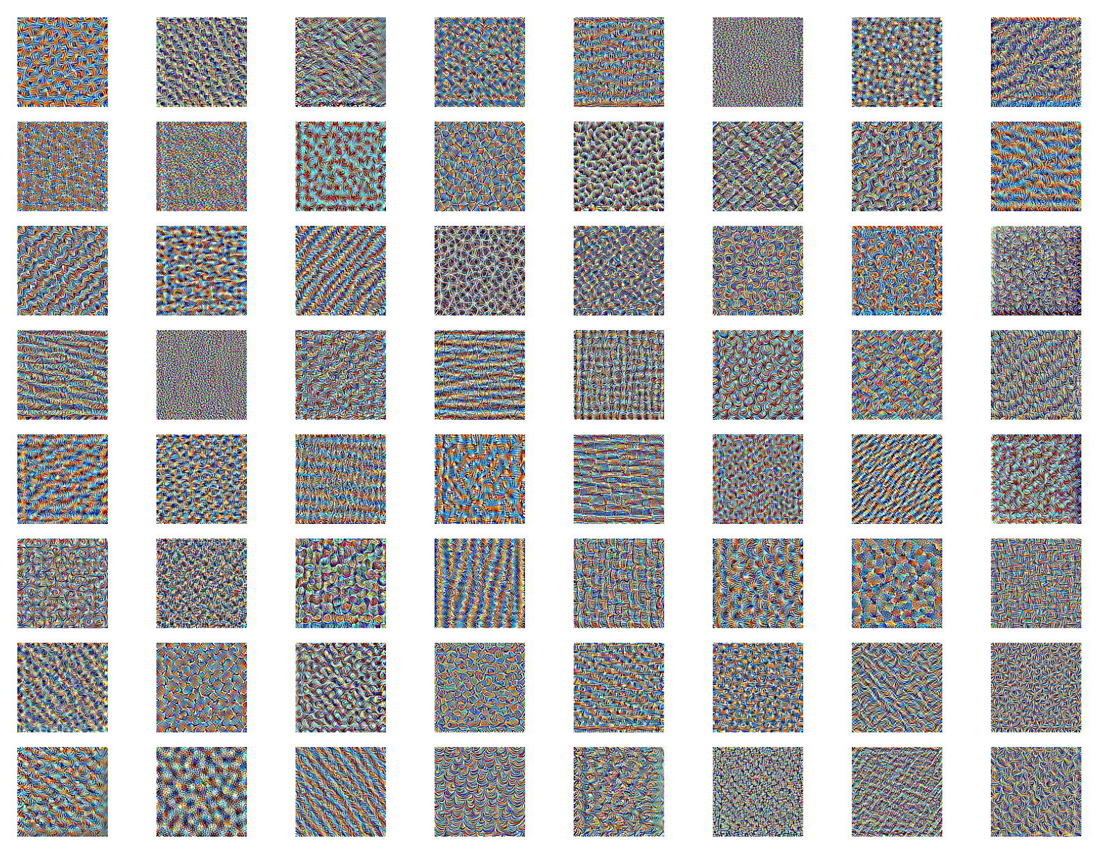
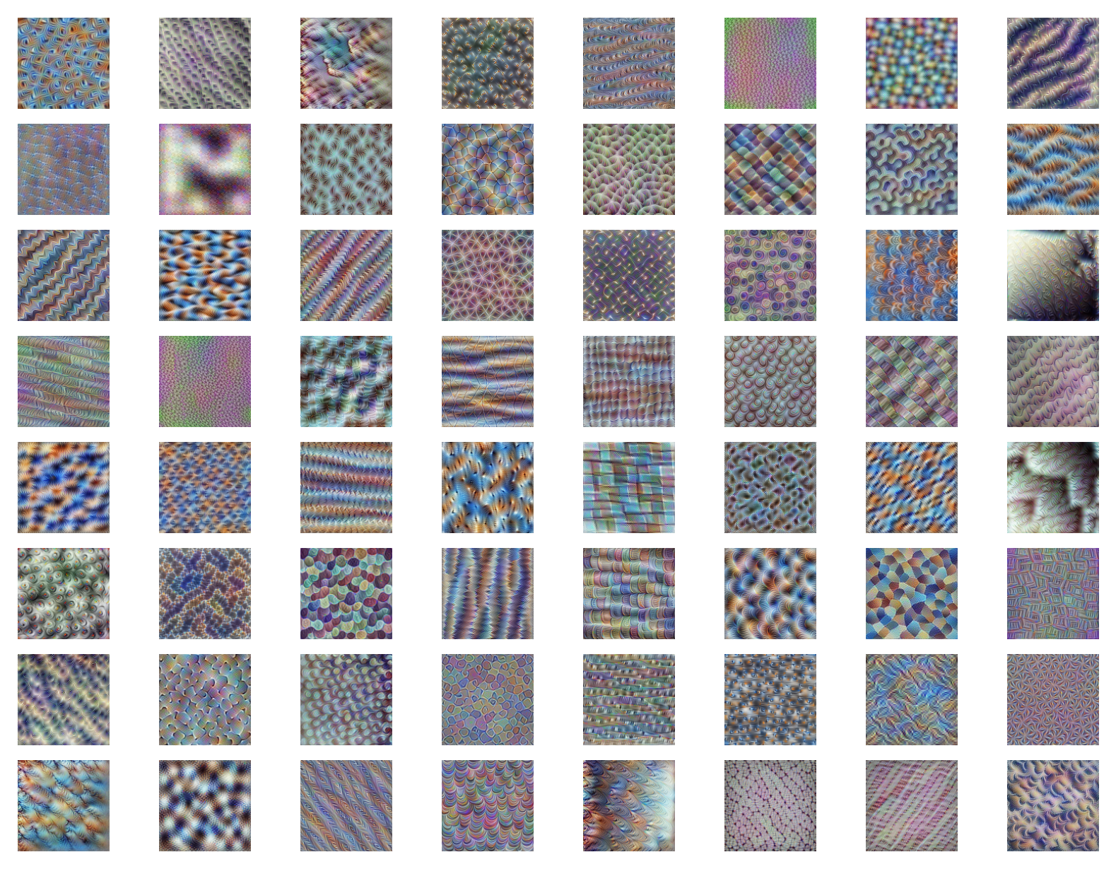
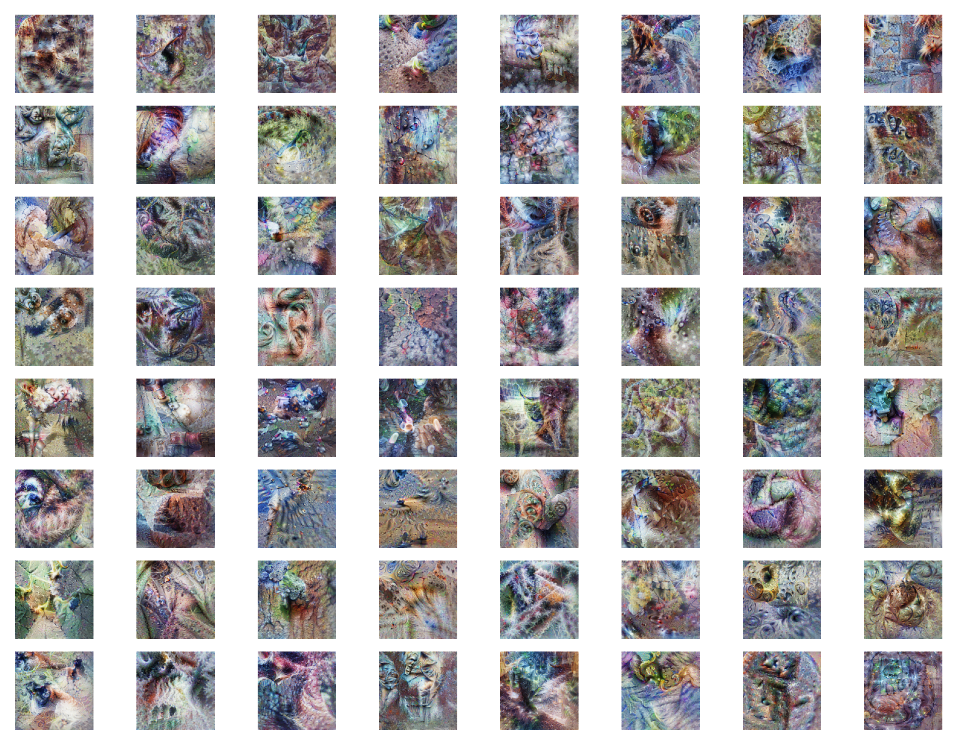
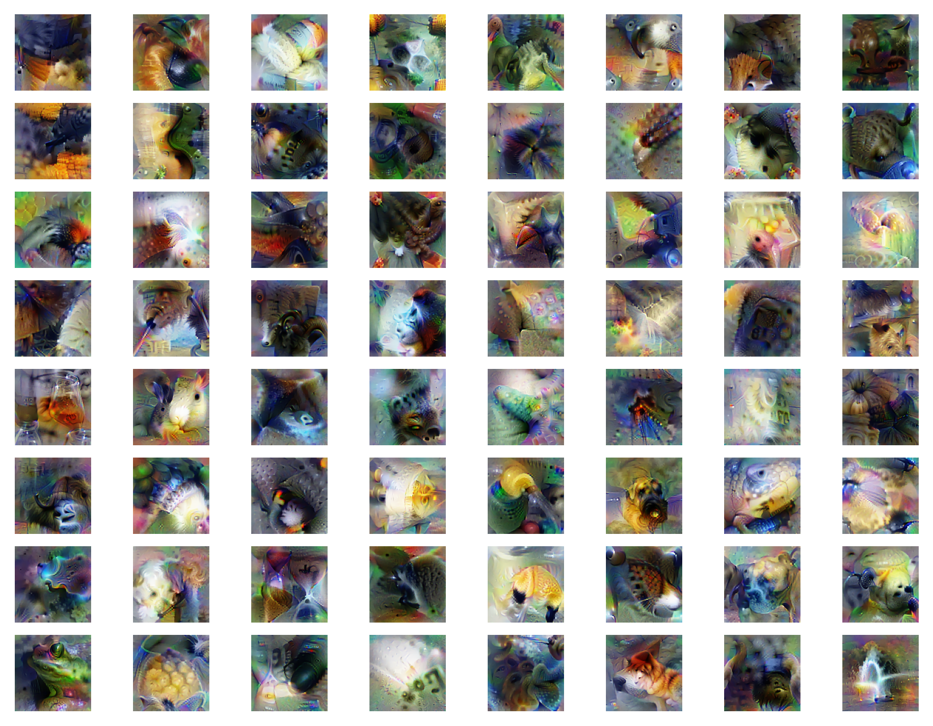
We start by looking at the low ResNet layer layer2.0.conv3. The feature visualisations we can see here demonstrate clear patterns which show a wider variety of ‘styles’ compared to the non-regularised versions. Comparing the regularised and non-regularised versions (which we can do because they’re the same filters from the same layer), we can see the similarities between the same features. Compared to the last post, these feature visualisations show less noise, more defined patterns and a greater variety of features!
Here are the old un-regularised feature visualisations (ResNet layer2.0.conv3):
Here are the newly (weakly) regularised feature visualisations (ResNet layer2.0.conv3):
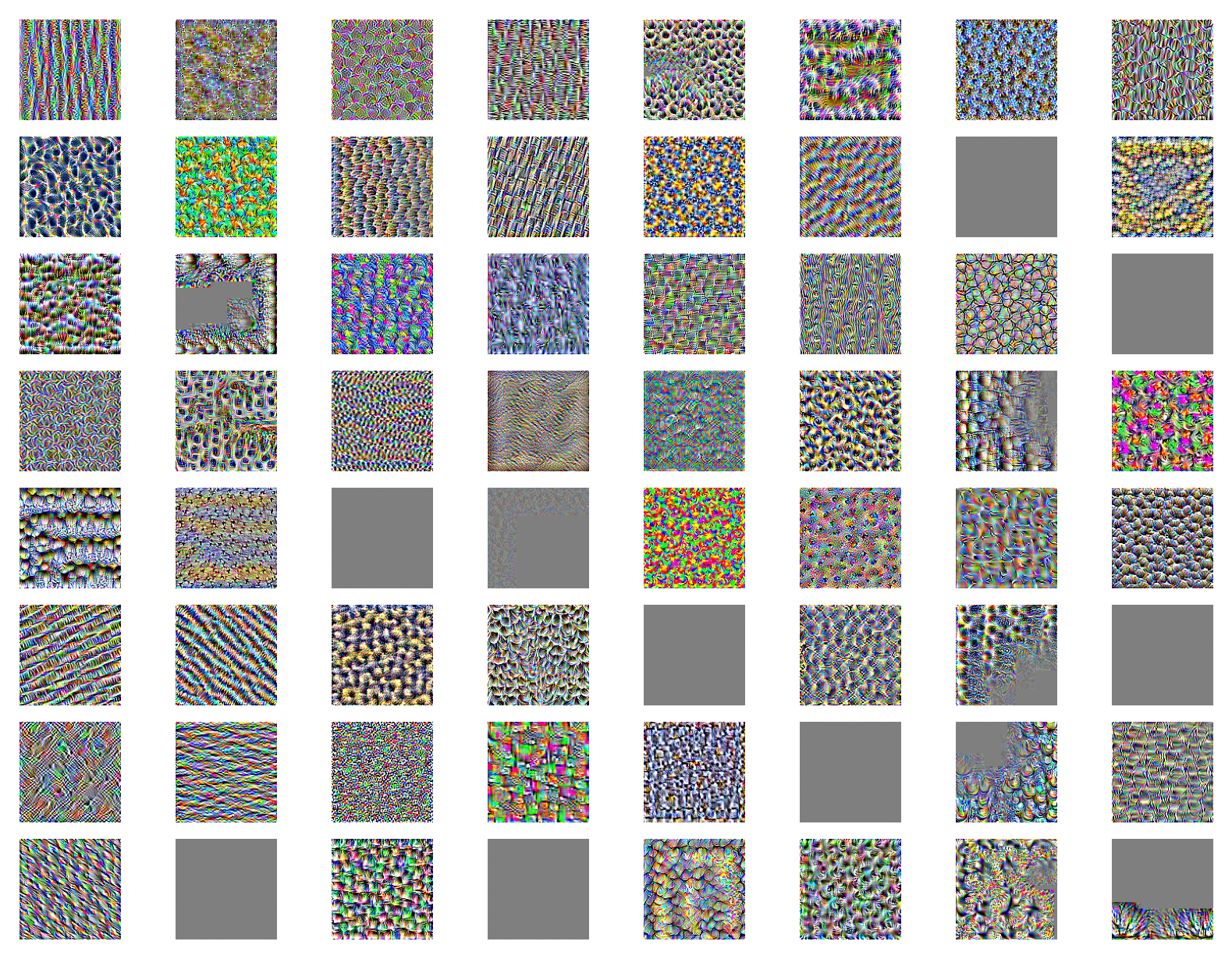
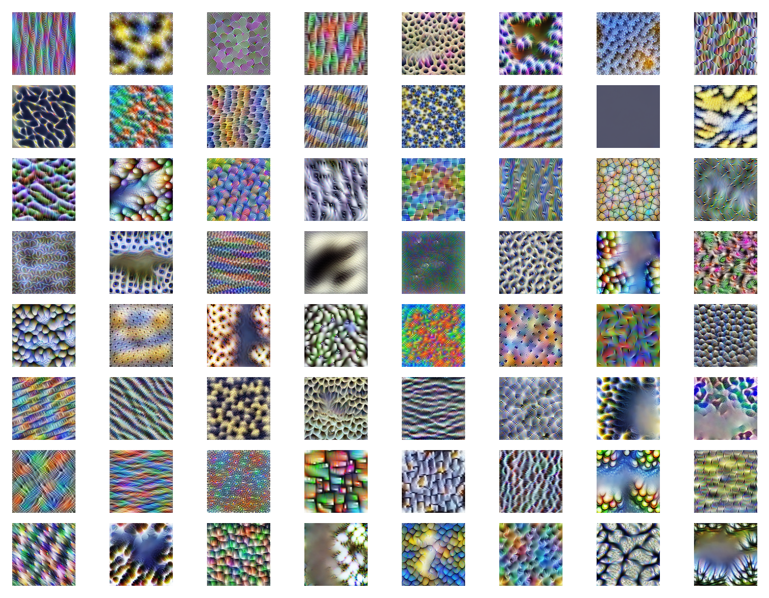
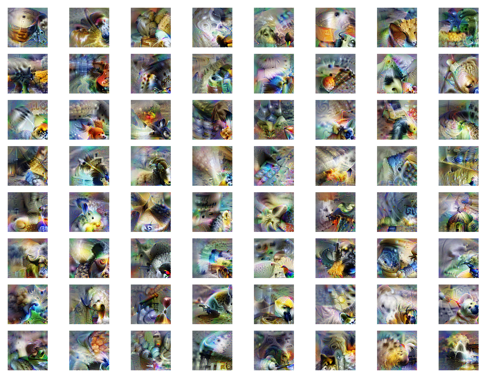
If we analyse a low layer of the GoogleNet architecture inception3b just as we did in the un-regularised approach we see a similar change in the visualised features as described for ResNet. We have less noise, more defined patterns and a greater variety of features once again!
Here are the old un-regularised feature visualisations (GoogleNet inception3b):
Here are the newly (weakly) regularised feature visualisations (GoogleNet inception3b):
Visualising higher level layers shows more complete structures with recognisable objects starting to emerge.
ResNet layer 4 convolution layer 3:
GoogleNet layer 4e:
Just out of interest I also generated some images which maximise individual neurons rather than channels. For GoogleNet inception5a.branch4[1].conv we get the following, rather cool, images:
Conclusion
I find feature visualisation a fascinating aspect of convolutional neural nets. Of course, the visual aspect is very cool, but the fact that we can gain a deeper understanding of what the network is learning is a very useful and enticing idea. Feature visualisation can be extended with neural circuits, which look at the connections between neurons and the features the neurons can generate and then try to explain the connections between them. An example from Zoom In: An Introduction to Circuits creates circuits where a dog head detector is built from neurons that detect oriented fur, then oriented dog heads, and the oriented dog heads combine to be orientation invariant!
This research has obvious applications to network interpretability. Seeing what a network is learning makes it possible to determine whether features are being extracted in a way in which we expect and make sure that networks are picking up on important discriminating features in a dataset rather than some unexpected property of a certain class of images (the (I believe debunked) parable of a military project detecting tanks from aerial images comes to mind where all images of tanks were taken on a cloudy day, and all images of non-tanks were sunny, the model performed poorly on new data, and it turns out they made a sunny vs cloudy day detector!). This deeper look into the inner workings of neural nets is important for systems where safety and security are critical! Any information we can extract about how these systems work allows us to be more confident in the system’s abilities and helps us avoid cases of unintended behaviour.
Resources
Again, this Distill article by Olah et al. is fantastic and is what the initial parts of this work was based on: Feature Visualization.
This is the Lucid library which supports Olah’s article with code. This helped my understanding of the topic and translation of the maths to code: Lucid - GitHub.
This is the Lucent library which is the PyTorch translation of Lucid. This also helped me understand some of the processes: Lucent: Lucid library adapted for PyTorch - GitHub.