Feature Visualisation Part 1 - Unregularised
Feature visualisation is a really helpful tool that can be used when trying to interpret what a neural network is actually learning under the hood. The process is incredibly simple: we pick a neuron we want to visualise, pass random noise as input to the network, ask the neuron to maximise its activation, and then backpropagate the changes that cause this maximal activation back to the input image. From this, we can effectively ‘see’ what the neuron is looking at (especially if we work with convolution neurons in the image space), which can help us to interpret what the network strongly responds to. In many image-based applications, this often leads to somewhat recognisable structures, which allow researchers to make conclusions about what a particular neuron activates for.
This simple description focuses on un-regularised features that often suffer from noise and focuses on high-frequency patterns, which oftentimes are not very interpretable to a human observer (however, the patterns do have interesting links to adversarial noise). This problem has a more complex solution, which I won’t discuss in this post. We’ll keep it simple for now and accept these high-frequency patterns as a stepping stone to a more robust and human-interpretable result.
The code
As is often the case in computer science, conceptual simplicity does not always entail implementation simplicity. This is also the case for feature visualisation. The code has been implemented as a colab notebook and aims to replicate the results found in this Keras tutorial, adapting the code to PyTorch.
The code starts out with a number of helper functions. view_available_layers takes a PyTorch model and gives a list of layers that we have access to and can be used for feature visualisation. It’s worth noting that not all layers are suited to feature visualisation, with convolution or batch norm layers often giving the best results.
We also have a function for generating random images (generate_random_image), which creates a completely grey image and adds some randomised noise in the R, G and B channels. This image acts as our original input to the model and is optimised to maximise the activation of the target.
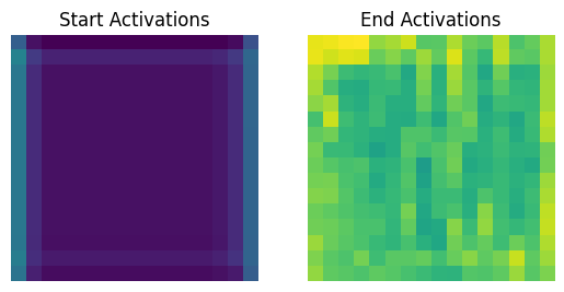
The display_activations function is a check to make sure that the optimisation is leading to increased activation. This essentially creates an image from the activations of the target before and after we optimise the image.
def view_available_layers(model):
    """
    Print all available layers for visualisation selection
    Parameters:
        - model (torch.nn.Module): The model to visualise the layer of
    """
    for name, layer in model.named_modules():
        print("{}".format(name))


def generate_random_image(shape=(3,128,128)) -> torch.Tensor:
    """
    Generate a random image with noise with a given number of channels, width and height
    Parameters:
        - shape (tuple of int, optional) - The width and height of the random image (default is (3, 128, 128))
    Returns:
        - image (torch.Tensor) - The image as a torch tensor
    """
    c,w,h = shape

    image = torch.ones(size=(1,c,w,h)) * 0.5
    noise = (torch.rand(size=(1, c, w, h))-0.5) * 0.005 # Was 0.05
    image += noise
    image.requires_grad = True
    return image


def display_activations(start_act, end_act):
    """
    Display the start and end activations
    Parameters:
        - start_act (numpy.ndarray): The activation matrix at the start of the optimisation process
        - end_act (numpy.ndarray): The activation matrix at the end of the optimisation process
    """
    fig, axes = plt.subplots(nrows=1, ncols=2)

    # Normalise the matrices between 0 and 1 for display
    # We need to do this across the two activations so we can see how they
    # change in relation to one another
    min = np.min(start_act) if np.min(start_act) < np.min(end_act) else np.min(end_act)
    max = np.max(start_act) if np.max(start_act) > np.max(end_act) else np.max(end_act)

    start_act += np.abs(min)
    start_act /= (np.abs(max) + np.abs(min) + 1e-5)
    end_act += np.abs(min)
    end_act /= (np.abs(max) + np.abs(min) + 1e-5)

    print("NORMALISED :: SA MAX: {} - SA MIN: {} - SA MEAN: {}".format(np.max(start_act), np.min(start_act), np.mean(start_act)))
    print("NORMALISED :: EA MAX: {} - EA MIN: {} - EA MEAN: {}".format(np.max(end_act), np.min(end_act), np.mean(end_act)))

    axes[0].set_title("Start Activations")
    axes[0].imshow(start_act, vmin=0, vmax=1)
    axes[0].axis('off')
    axes[1].set_title("End Activations")
    axes[1].imshow(end_act, vmin=0, vmax=1)
    axes[1].axis('off')
    plt.show()
We then have the visualisation loss VisLoss which provides a metric which guides the optimisation. This loss takes the mean of the activation and returns the negative of the result since we aim to maximise it.
class VisLoss(torch.nn.Module):
    """
    Define a new loss function for visualisation
    """
    def forward(self, activation):
        """
        Overrides the default forward behaviour of torch.nn.Module
        Parameters:
            - activation (torch.Tensor): The activation tensor after the network function has been applied to the image
        Returns:
            - (torch.Tensor): The mean of the activation tensor (avoiding the border to reduce artefacts)
        """
        return -activation.mean()
Next is the visualisation code hook_visualise. This starts by setting the model to eval mode (which is a really important part of the process and something that I missed and spent longer than I care to admit debugging). We then set up and register the forward hook for the activation, which basically sets a listener at the target layer, so when we pass forward through the model, we grab the activation results at the target layer and can process them later. We then define a whole lot of variables, including the optimisation image, the loss function, the optimiser (ADAM), and many activations and losses to keep track of the best-performing image. Next, the optimisation process starts. As with all optimisation, we start by zeroing the optimiser gradient. Then, we pass the optimisation image to the model (ignoring the results). We check the type of optimisation we want to perform from layer/dream- where we optimise over the entire layer of the network (i.e. all channels of the convolution), channel- (the default) where we optimise over a single channel, or neuron- where we optimise over a single neuron only. All images generated for this post were created using the channel option. We then calculate the loss, backpropagate, and then take a step in the direction specified by the optimiser. The rest of the code in this function is just bookkeeping, checking the losses to ensure we return the image with the best loss and updating the activation images and losses we store along the way.
def hook_visualise(model, target, filter, iterations=30, lr=10.0, opt_type='channel'):
    """
    Visualise the target layer of the model
    Parameters:
    - model (torch.nn.Module): The model to visualise a layer of
    - target (str): The target layer to visualise
    - filter (int): The target filter/kernel to visualise
    - iterations (int, optional): The number of optimisation iterations to run for (default is 30)
    - lr (float, optional):  The learning rate for image updates (default is 10.0)
    - opt_type (str, optional): The type of optimisation (neuron, channel, layer/dream) (default is 'channel')
    """
    # Set the model to evaluation mode - SUPER IMPORTANT
    model.eval()

    global activation
    activation = None
    def activation_hook(module, input, output):
        global activation
        activation = output

    hook = target.register_forward_hook(activation_hook)

    # Create the random starting image
    image = generate_random_image(shape=(3,128,128))
    image = image.detach()
    image.requires_grad = True

    # Define the custom loss function
    loss_fn = VisLoss()

    opt = torch.optim.Adam(params=[image], lr=lr)

    history = {"mean":[], "max":[], "min":[], "loss":[]}
    start_act = None
    end_act = None
    best_act = None
    best_loss = np.inf
    best_image = None
    best_it = 0

    max_iterations = iterations
    for it in range(max_iterations):

        opt.zero_grad()

        _ = model(image)

        if opt_type == 'layer' or opt_type == 'dream':
            act = activation[0, :, :, :] # Layer (DeepDream)
        elif opt_type == 'channel':
            act = activation[0, filter, :, :] # Channel
        elif opt_type == 'neuron':
            # Select the central neuron by default
            nx, ny = activation.shape[2], activation.shape[3]
            act = activation[0, filter, nx//2, ny//2] # Neuron

        loss = loss_fn(act)

        loss.backward()
        opt.step()

        if loss < best_loss:
            best_loss = loss
            best_image = image.clone()
            best_act = act.detach().numpy()
            best_it = it+1


        print("Iteration: {}/{} - Loss: {:.3f}".format(it+1, max_iterations, loss.detach()))
        np_act = act.detach().numpy()
        if it == 0:
            start_act = np_act
        if it == max_iterations-1:
            end_act = np_act
        print("ACT - Mean: {:.4f} - STD: {:.4f} - MAX: {:.4f} - MIN: {:.4f} - Loss: {:.4f}".format(np.mean(np_act), np.std(np_act), np.max(np_act), np.min(np_act), loss))
        history["mean"].append(np.mean(np_act))
        history["max"].append(np.max(np_act))
        history["min"].append(np.min(np_act))
        history["loss"].append(loss.detach().numpy())

    print("Best loss: {} - Iteration: {}".format(best_loss, best_it))
    optimized_image = best_image.detach().squeeze().cpu()
    optimized_image = optimized_image.permute(1,2,0)

    pre_inv = optimized_image.clone()
    optimized_image = torch.clamp(optimized_image, 0, 1)
    pre_inv = torch.clamp(pre_inv * 255, 0, 255).to(torch.int)

    hook.remove() # Remove the hook so subsequent runs don't use the previously registered hook!

    return init_image, history, start_act, best_act, optimized_image, pre_inv
The code in the colab notebook focuses on two architectures ResNet-50 and GoogleNet, but can be adapted to any architecture.
Feature visualisations
The following image strongly activates ResNet at the convolution layer layer2.0.conv3, filter 0. The corresponding activation change can be seen below it!
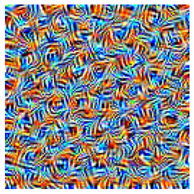
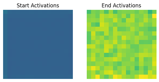
As these images show, the feature visualisation process is able to cause increased activation at the convolution filter specified, which results in a patterned image.
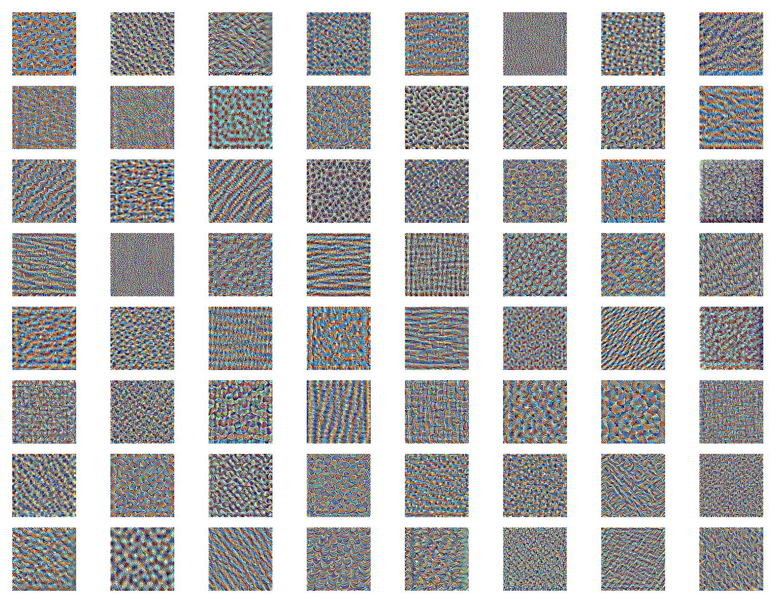
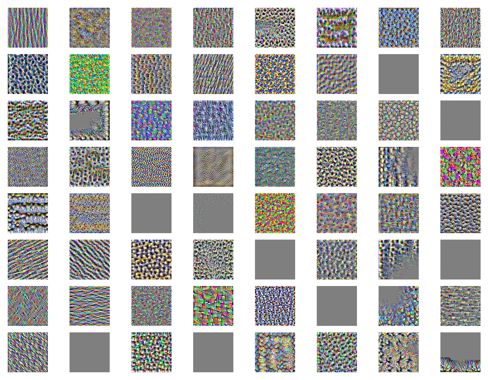
If we expand this to look at the first 64 features, we get the following images which are reminicient of the Keras tutorial referenced earlier.
If we look at the images produced by GoogleNet, we can see the features extracted by this method. First, the Inception 3B layer focusing on filter 0 shows:
With the activation images:
Expanding this to the first 64 filters of 3B leads to these features:
Within the features above we can see some grey images where the optimisation process has failed to find a good direction to move in, with some features having blocks of grey which is an interesting effect! These failures can be addressed with more complex regularised feature visualisation processes.
The extracted features above focus on fairly early layers from ResNet and GoogleNet. What about later (higher level) layers?
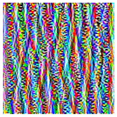
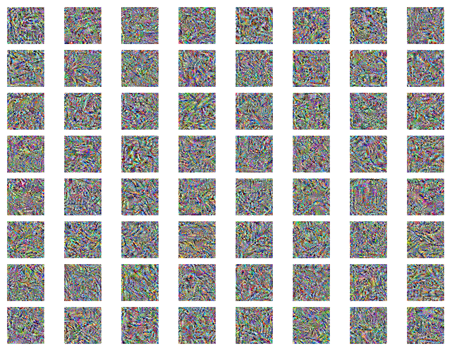
The ResNet layer 4 convolution 3 target produces the feature visualisations shown below.
With GoogleNet layer 4e here.
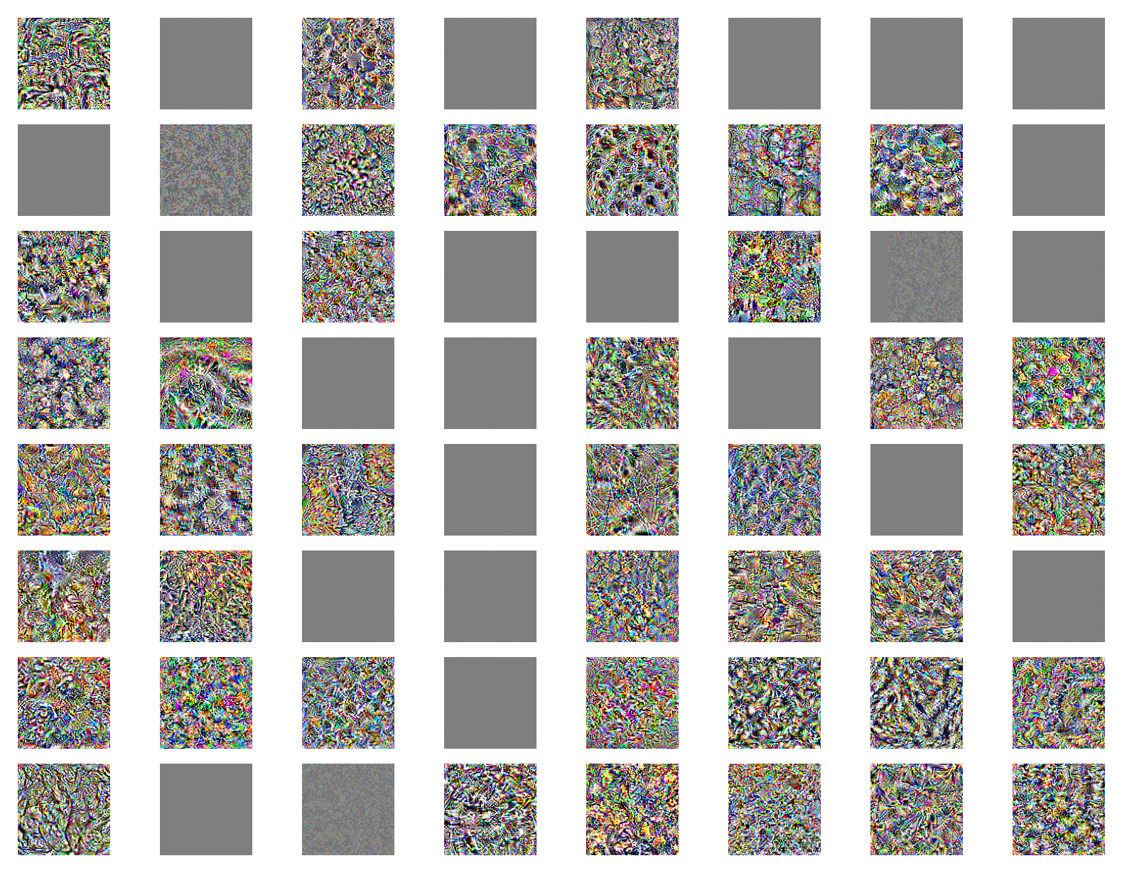
In both instances we see high frequency noisy patterns which don’t really resemble anything that we as humans would be able to identify in relation to the classification task (e.g. there are no images which reference cats, dogs, cars or planes). At the later stages of the networks, which we get these features from, we’d expect to see something at least vaguely recognisable.
This approach to feature visualisation is a good start when we’re trying to determine what networks ‘see’ and gain some insight into the classification process. However, the high frequency patterns leave a lot to be desired when we’re trying to understand the behaviour of a network and how classifications are produced (especially at the higher layers of the network). This leads us to regularised feature visualisation approaches which generate insights which are more human interpretable. Details on regularised approaches can be found in the next post!
In addition, this approach to feature visualisation focuses on individual neurons/channels, and since neural networks consist of many hundreds of thousands/millions of neurons, we only get a small slice of the information. In addition, these feature visualisations often occur with no dependency on previous neurons (each neuron in each layer is maximised in isolation) and since neural networks are incredibly connected structures, this may not give the best indication of the relationship of a neuron to others in the network structure. To expand on this feature visualisation technique, neural circuits are used; however, that’s another story.
Resources
The Keras implementation can be found here.
The post by Olah et al. which started all of this (and is a really useful resource for all things interpretability based) can be found here.